How CamForge corrects discontinuities in cam SVAJ curves

A cam may be assembled from individually valid segments and still present jumps at their junctions. CamForge corrects this problem by using continuity equations to redistribute angular intervals or displacements without replacing the selected motion laws.

The equation of an SVAJ segment

Consider segment \(i\), starting at \(\theta_i\), with angular interval \(\beta_i\) and displacement change \(\Delta L_i\). A local dimensionless coordinate is defined so that it always varies from 0 to 1:

\[ u_i=\frac{\theta-\theta_i}{\beta_i},\qquad 0\leq u_i\leq1. \]

If \(f_i(u)\) is the normalized motion law, with \(f_i(0)=0\) and \(f_i(1)=1\), displacement is:

\[ S_i(\theta)=L_i+\Delta L_i\,f_i(u_i). \]

The chain rule gives the remaining SVAJ curves:

\[ S_i'=\frac{\Delta L_i}{\beta_i}f_i'(u_i),\qquad S_i''=\frac{\Delta L_i}{\beta_i^2}f_i''(u_i),\qquad S_i'''=\frac{\Delta L_i}{\beta_i^3}f_i'''(u_i). \]

These derivatives are velocity, acceleration and jerk with respect to cam angle. At constant angular speed \(\omega\), their time-domain counterparts are \(v=\omega S'\), \(a=\omega^2S''\) and \(j=\omega^3S'''\). Therefore, continuity in \(S'\) and \(S''\) also provides continuous physical velocity and acceleration.

Mathematical conditions at a junction

Between segments \(i\) and \(i+1\), displacement, velocity and acceleration continuity require:

\[ S_i(\theta_i+\beta_i)=S_{i+1}(\theta_{i+1}), \] \[ \frac{\Delta L_i}{\beta_i}f_i'(1) = \frac{\Delta L_{i+1}}{\beta_{i+1}}f_{i+1}'(0), \] \[ \frac{\Delta L_i}{\beta_i^2}f_i''(1) = \frac{\Delta L_{i+1}}{\beta_{i+1}^2}f_{i+1}''(0). \]

The first equality follows from \(L_{i+1}=L_i+\Delta L_i\). The other two depend on the motion law, \(\Delta L\), and \(\beta\). Let the endpoint coefficients be:

\[ c^V_{i,0}=f_i'(0),\quad c^V_{i,f}=f_i'(1),\qquad c^A_{i,0}=f_i''(0),\quad c^A_{i,f}=f_i''(1). \]

These coefficients are known numbers for each motion law. If one side requires a zero derivative and the other a nonzero derivative, changing only \(\beta\) or \(\Delta L\) cannot satisfy the equation. When zeros and signs are compatible, the equations determine the correction.

Correction by changing only β

All \(\Delta L_i\) remain fixed and the unknowns are the angular intervals. Velocity continuity directly gives:

\[ \boxed{ \frac{\beta_{i+1}}{\beta_i} = \frac{\Delta L_{i+1}c^V_{i+1,0}} {\Delta L_i c^V_{i,f}} }. \]

When acceleration controls the junction:

\[ \boxed{ \frac{\beta_{i+1}}{\beta_i} = \sqrt{ \frac{\Delta L_{i+1}c^A_{i+1,0}} {\Delta L_i c^A_{i,f}} } }. \]

The quantity under the square root must be positive. The valid ratios allow all angles to be written in terms of one unknown:

\[ \beta_2=r_2\beta_1,\quad \beta_3=r_3\beta_1,\quad\ldots,\quad \beta_n=r_n\beta_1. \]

The full revolution condition determines the scale:

\[ \sum_{i=1}^{n}\beta_i=360^\circ \quad\Longrightarrow\quad \beta_1=\frac{360^\circ}{1+r_2+r_3+\cdots+r_n}. \]

Correction by changing only ΔL

The angles remain fixed and the displacement changes are the unknowns. Continuity becomes linear because every denominator is known:

\[ \boxed{ \frac{c^V_{i,f}}{\beta_i}\Delta L_i - \frac{c^V_{i+1,0}}{\beta_{i+1}}\Delta L_{i+1}=0 }, \] \[ \boxed{ \frac{c^A_{i,f}}{\beta_i^2}\Delta L_i - \frac{c^A_{i+1,0}}{\beta_{i+1}^2}\Delta L_{i+1}=0 }. \]

Returning to the initial position adds the cycle-closure equation:

\[ \boxed{\sum_{i=1}^{n}\Delta L_i=0}. \]

Together, these equations form a homogeneous linear system:

\[ A\,\boldsymbol{\Delta L}=\mathbf 0,\qquad \boldsymbol{\Delta L}= \begin{bmatrix}\Delta L_1&\Delta L_2&\cdots&\Delta L_n\end{bmatrix}^{T}. \]

An equivalent form, used by CamForge, works with displacement levels \(L_i\), where \(\Delta L_i=L_{i+1}-L_i\) and \(L_n=L_0\). The continuity equations can then be collected as \(A\mathbf L=\mathbf b\). When more than one solution exists, the one closest to the original levels \(\mathbf L^{(0)}\) is selected:

\[ \min_{\mathbf L}\; \frac{1}{2} \left(\mathbf L-\mathbf L^{(0)}\right)^T W \left(\mathbf L-\mathbf L^{(0)}\right) \qquad \text{subject to}\qquad A\mathbf L=\mathbf b. \]

The diagonal matrix \(W\) balances changes in strokes of different magnitudes. With Lagrange multipliers \(\boldsymbol{\lambda}\), the minimum conditions are written as:

\[ \begin{bmatrix} W & A^T\\ A & 0 \end{bmatrix} \begin{bmatrix} \mathbf L\\ \boldsymbol{\lambda} \end{bmatrix} = \begin{bmatrix} W\mathbf L^{(0)}\\ \mathbf b \end{bmatrix}. \]

The corrected strokes follow from \(\Delta L_i=L_{i+1}-L_i\). They satisfy velocity, acceleration and closure, preserve every \(\beta_i\), and remain as close as possible to the initially specified motion.

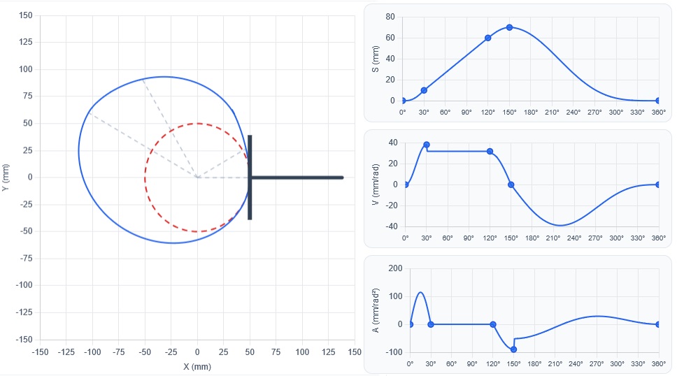
In short: changing only β redistributes the angle available to the same strokes; changing only ΔL redistributes the strokes within the same angular intervals. Both modes start from the same continuity equations.

Example: four incompatible segments

Segment	β	ΔL	Curve
1	30°	10 mm	C1 — cycloidal first half
2	90°	50 mm	VC — constant velocity
3	30°	10 mm	H2 — harmonic second half
4	210°	−70 mm	DH — double-harmonic return

Cumulative displacement passes through 0, 10, 60 and 70 mm before returning to zero. Position closes correctly, but velocity jumps at C1–VC and VC–H2, while acceleration jumps at H2–DH.

Figure 1 — Initial profile and SVA diagrams. Displacement is continuous, but velocity and acceleration jump at segment boundaries.

Applying the equations

The normalized equations of the first three segments are:

\[ f_{\mathrm{C1}}(u)=u-\frac{\sin(\pi u)}{\pi},\qquad f_{\mathrm{VC}}(u)=u,\qquad f_{\mathrm{H2}}(u)=\sin\left(\frac{\pi u}{2}\right). \]

The required endpoint coefficients are:

\[ f_{\mathrm{C1}}'(1)=2,\quad f_{\mathrm{VC}}'(0)=f_{\mathrm{VC}}'(1)=1, \] \[ f_{\mathrm{H2}}'(0)=\frac{\pi}{2},\quad f_{\mathrm{H2}}'(1)=0,\quad f_{\mathrm{H2}}''(1)=-\frac{\pi^2}{4}. \]

For the double-harmonic return, \(f_{\mathrm{DH}}'(0)=0\) and \(f_{\mathrm{DH}}''(0)=\pi^2\). Since \(\Delta L_4=-70\) mm, its initial acceleration is negative, matching the sign at the end of H2.

Velocity continuity at C1–VC gives:

\[ \frac{10(2)}{\beta_1}=\frac{50(1)}{\beta_2} \quad\Longrightarrow\quad \beta_2=2.5\beta_1. \]

At VC–H2:

\[ \frac{50(1)}{\beta_2}=\frac{10(\pi/2)}{\beta_3} \quad\Longrightarrow\quad \beta_3=\frac{\pi}{10}\beta_2=\frac{\pi}{4}\beta_1. \]

Velocity is zero on both sides of H2–DH, so acceleration determines the ratio:

\[ \frac{10(-\pi^2/4)}{\beta_3^2} = \frac{-70(\pi^2)}{\beta_4^2} \quad\Longrightarrow\quad \beta_4=\sqrt{28}\,\beta_3. \]

The angular closure equation is:

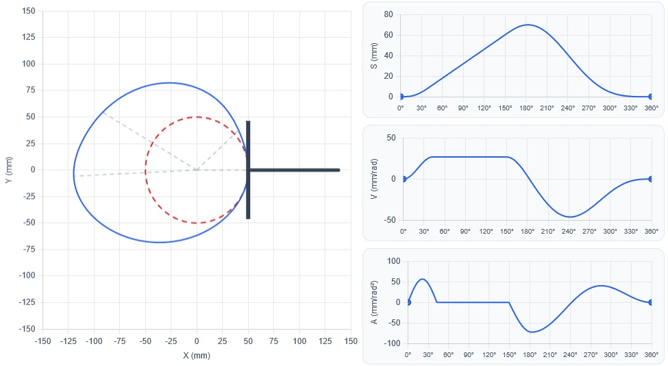
\[ \beta_1+2.5\beta_1+\frac{\pi}{4}\beta_1 +\sqrt{28}\frac{\pi}{4}\beta_1=360^\circ. \]

Segment	Original β	Corrected β	Preserved ΔL	Curve
1	30°	42.65°	10 mm	C1
2	90°	106.62°	50 mm	VC
3	30°	33.49°	10 mm	H2
4	210°	177.24°	−70 mm	DH

Before rounding, the angles are approximately 42.64728°, 106.61821°, 33.49509° and 177.23940°. Any small discrepancy in the rounded sum is due only to displaying two decimal places.

Figure 2 — Result after “Change beta only.” Velocity and acceleration cross the boundaries without jumps, and the cam profile is smoother.

A bottleneck resolved in moments

Doing this by hand requires differentiating every motion law, evaluating endpoints, writing the equalities, closing the 360° cycle and recalculating the profile. With many segments, this compatibility work becomes a bottleneck between motion definition and geometric cam analysis.

CamForge applies these equations almost instantly and presents a continuous configuration directly. The designer still decides which motions and constraints make engineering sense, but no longer needs to repeat lengthy algebraic compatibility calculations. The path from an SVAJ specification to a smooth cam profile becomes much faster.